Manipulation
This is a course project for Robot Modeling and Control. [report]
In this project, we aim to control the robotic arm to transport the four blocks from the starting place through the dyeing pool to the destination and place them according to the requirement.
The phases of the movement process can be divided into linear movement phases ( $q_{left}$ -> $q_{right}$) and non-linear movement phases, and the two different types of phases need to use different trajectory planning methods as shown below.
Non-linear trajectory planning
For this type of trajectory planning, we use the quintic polynomial solution:
\[q(t) = a_{0} + a_{1} t + a_{2} t^{2} + a_{3} t^{3} + a_{4} t^{4} + a_{5} t^{5}\]The constraints are:
\[\begin{cases} q(0) = q_{0} \\ q(t) = q_{f} \\ q'(0) = q_{0}' \\ q'(t) = q_{f}' \\ q''(0) = q_{0}'' \\ q''(t) = q_{f}'' \end{cases}\]Hence, the following equation can be obtained:
\[\begin{pmatrix} t_{0}^{5} & t_{0}^{4} & \cdots & 1 \\ t_{f}^{5} & t_{f}^{4} & \cdots & 1 \\ 5 t_{0}^{4} & 4 t_{0}^{3} & \cdots & 0 \\ 5 t_{f}^{4} & 4 t_{f}^{3} & \cdots & 0 \\ 20 t_{0}^{3} & 12 t_{0}^{2} & \cdots & 0 \\ 20 t_{f}^{3} & 12 t_{f}^{2} & \cdots & 0 \end{pmatrix} \begin{pmatrix} a_{0} \\ a_{1} \\ a_{2} \\ a_{3} \\ a_{4} \\ a_{5} \end{pmatrix} = \begin{pmatrix} \boldsymbol{q}_{0} \\ \boldsymbol{q}_{f} \\ \boldsymbol{q}_{0}' \\ \boldsymbol{q}_{f}' \\ \boldsymbol{q}_{0}'' \\ \boldsymbol{q}_{f}'' \end{pmatrix}\]The coefficients of the quintic polynomial can be obtained by solving the matrix equation. We can get the joint angles of the robotic arm at any time by substituting the time t into the quintic polynomial function.
The above procedures are shown in function trajPlanningDemo() as follows.
def trajPlaningDemo(start, end, t, time):
    """ Quintic Polynomial: x = k5*t^5 + k4*t^4 + k3*t^3 + k2*t^2 + k1*t + k0
    :param start: Start point
    :param end: End point
    :param t: Current time
    :param time: Expected time spent
    :return: The value of the current time in this trajectory planning
    """
    if t < time:
        tMatrix = np.matrix([
        [         0,           0,             0,          0,        0,   1],
        [   time**5,     time**4,       time**3,    time**2,     time,   1],
        [         0,           0,             0,          0,        1,   0],
        [ 5*time**4,   4*time**3,     3*time**2,     2*time,        1,   0],
        [         0,           0,             0,          2,        0,   0],
        [20*time**3,  12*time**2,        6*time,          2,        0,   0]])

        xArray = []
        for i in range(len(start)):
            xArray.append([start[i], end[i], 0, 0, 0, 0])
        xMatrix = np.matrix(xArray).T

        kMatrix = tMatrix.I * xMatrix

        timeVector = np.matrix([t**5, t**4, t**3, t**2, t, 1]).T
        x = (kMatrix.T * timeVector).T.A[0]

    else:
        x = end

    return x
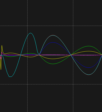
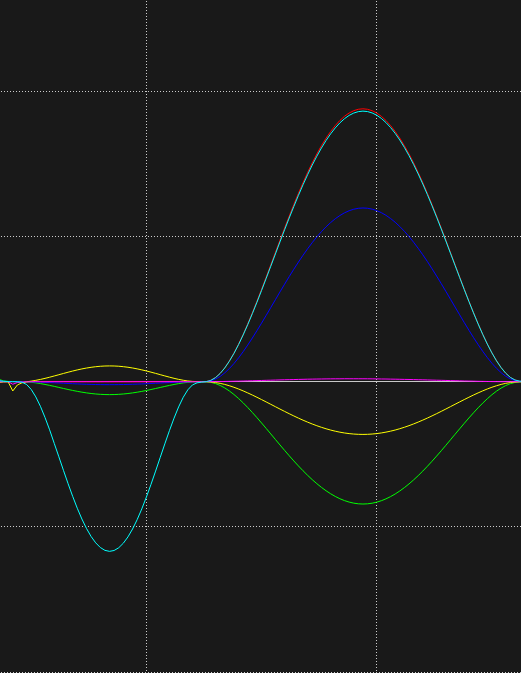
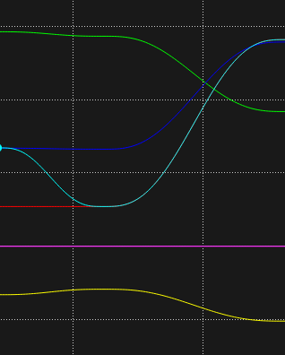
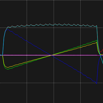
The non-linear segments of the curves are depicted below. Since we use the quintic polynomial to do trajectory planning, the velocity of the joint angles is a quartic polynomial while the acceleration is a cubic polynomial. So they are both smooth curves without sharp changes.
Linear trajectory planning
Linear trajectory planning restricts the positional changes of the robotic arm in the world coordinate system. Here we use the segmented sampling method, where the straight line is segmented first, and the joint angles of each point on the line can be obtained using the IK solver.
Due to the large number of segments, the position change of each segment is very small, so we can directly use the move() function to move the robotic arm from one end of the segment to the other one by one, which in the end enables the robotic arm to move in a straight line.
def LineartrajPlanning(start, end, t, time):
    if t < time:
        r = int(t / time * num_line_points)
        res = spline_q_lists[r]
    else:
        res = spline_q_lists[num_line_points-1]

    if True in np.isnan(res):
        print("trajPlaning(): NAN")
        return False
    return res
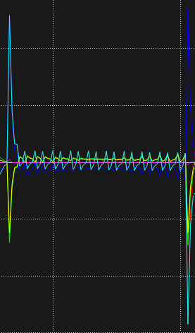
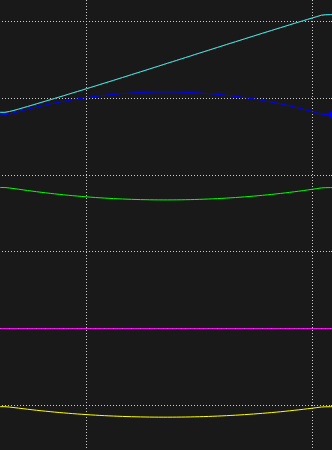
The linear segments of the curves are depicted as follows. We adopted the segmented sampling method, so we can see that the velocity and acceleration curves fluctuate regularly. Since this is a uniform motion, the acceleration curve exhibits slight fluctuations near zero, while the velocity curve shows minor variations around the predetermined velocity value. The joint position transitions smoothly, resembling a roughly linear process.
Real World Test
This is how our algorithm performs in a real world test: